A Basic Introduction to Additive White Gaussian Noise
Abstract: This document provides a basic introduction to thermal noise and Additive White Gaussian Noise (AWGN), including its main characteristics, how AWGN can be generated, and how calibrated noise sources are used for noise figure measurements.
Please click here to download the document as a PDF file.
Thermal noise is everywhere. It exists in every system and every circuit within a system. And because of the randomness of its nature it cannot be cancelled out. In 1926 at Bell Labs in New York, John B. Johnson investigated ways of detecting and measuring thermal noise, and the theory behind it was later explained by his colleague Harry Nyquist. Thermal noise, also known as Johnson-Nyquist Noise, is naturally occurring and caused by the thermal agitation of charge carriers, usually electrons, inside an electrical conductor. Hence everything with a temperature above 0 Kelvin, or absolute zero, emits thermal noise.
As technology has progressed, the problem of how to deal with noise has become more and more challenging to design engineers in a wide range of industries. Performance can be improved by cooling the receiver circuitry in order to lower the noise floor, but in most applications this is not possible. Lower signal levels, complex modulation schemes and increasingly sensitive receivers mean that there is a greater chance of a system’s performance being adversely affected by thermal noise.
The thermal noise power N of a noise source is given by:
N(Watts) = kTB
where k is the Boltzmann constant (1.38 x 10⁻²³ J/K), T is temperature (Kelvin), and B is bandwidth (Hz).
From this equation the thermal noise floor is found to be -174dBm/Hz at a temperature of 290 K, which is universally accepted as the average temperature of the Earth’s surface. This value is used as a reference level when carrying out noise figure calculations.
Additive White Gaussian Noise (AWGN) is a close approximation to thermal noise. Its advantage is that it can be generated and precisely controlled in order to produce specifically defined levels over the bandwidths of interest. So devices which create such signals are useful for simulating how a system performs in the real world.
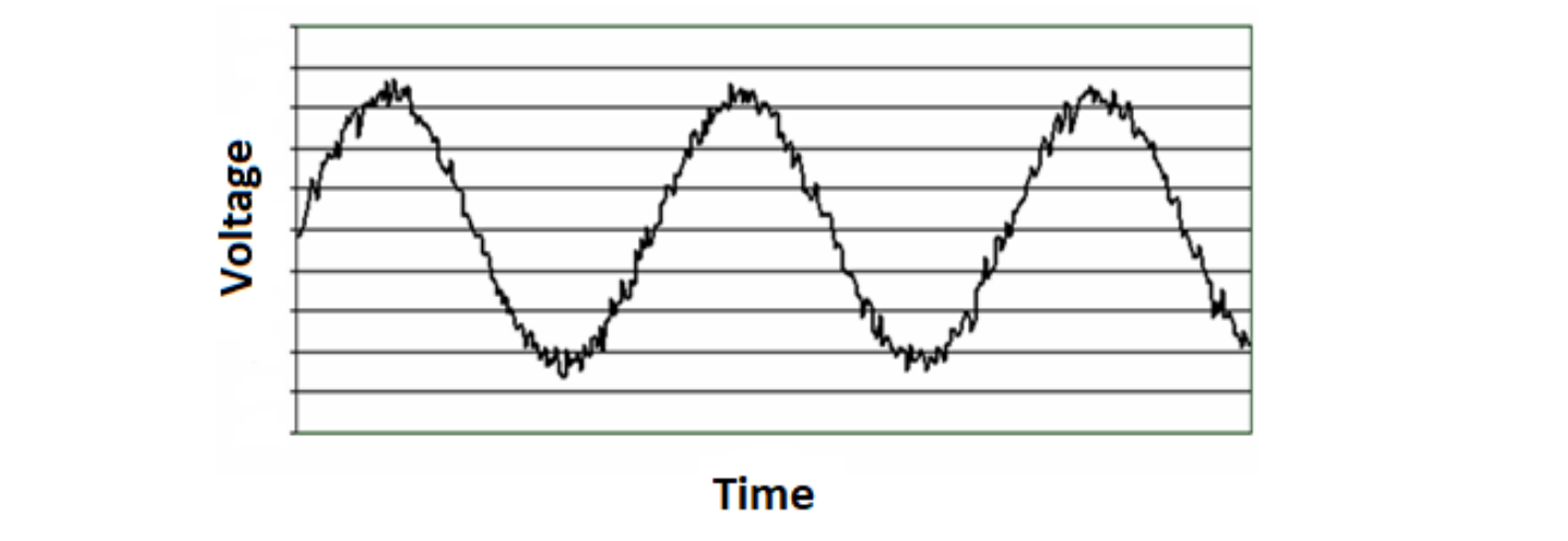
Additive – This indicates that the noise is simply added to the transmitted signal to give signal plus noise. An oscilloscope would display such a signal in the following way.
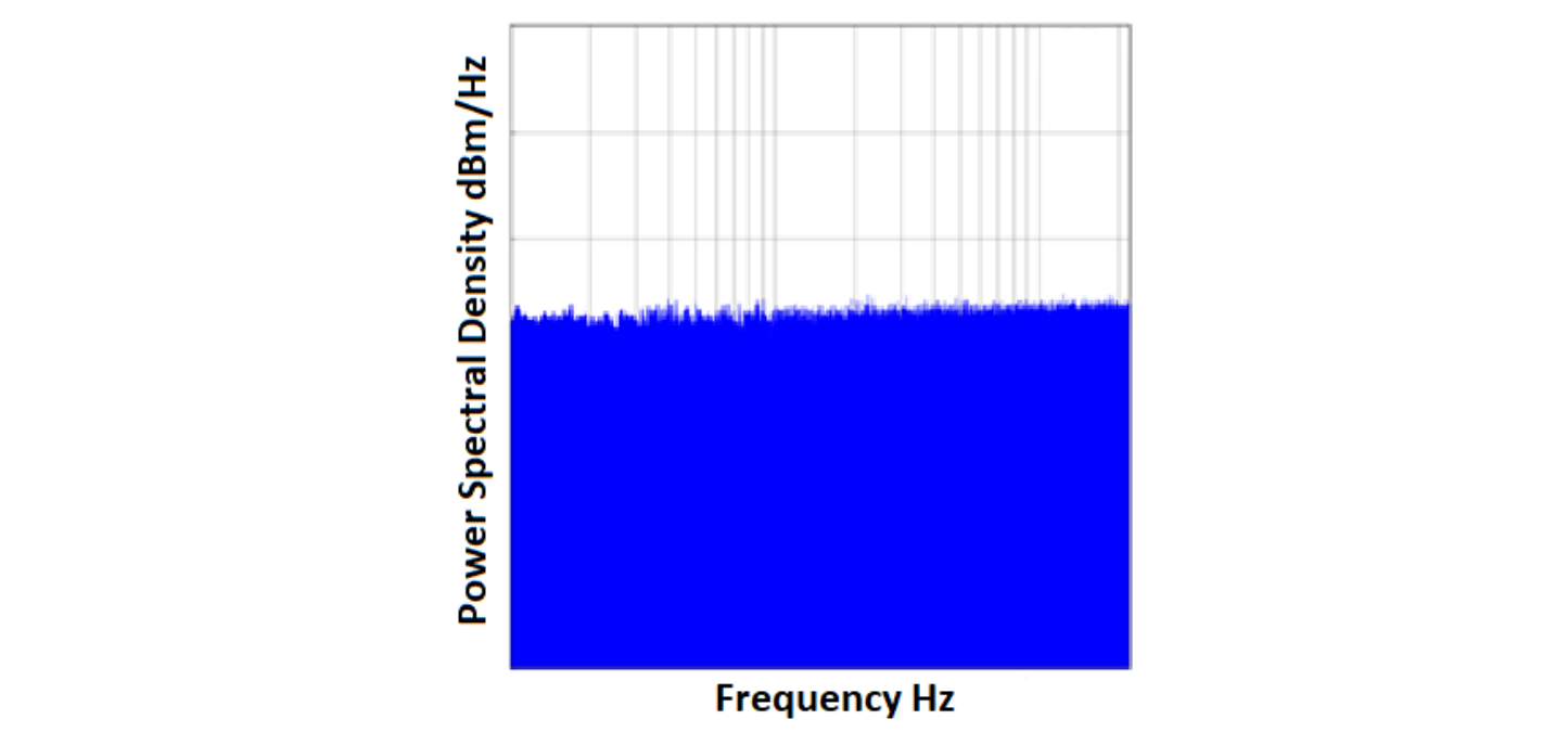
White – The noise has the same power distribution at any frequency across its band. On a spectrum analyser a flat line will therefore be displayed, as shown below.
The power distribution of the noise is approximately Gaussian, and so follows the classic bell shaped curve in the statistical domain.
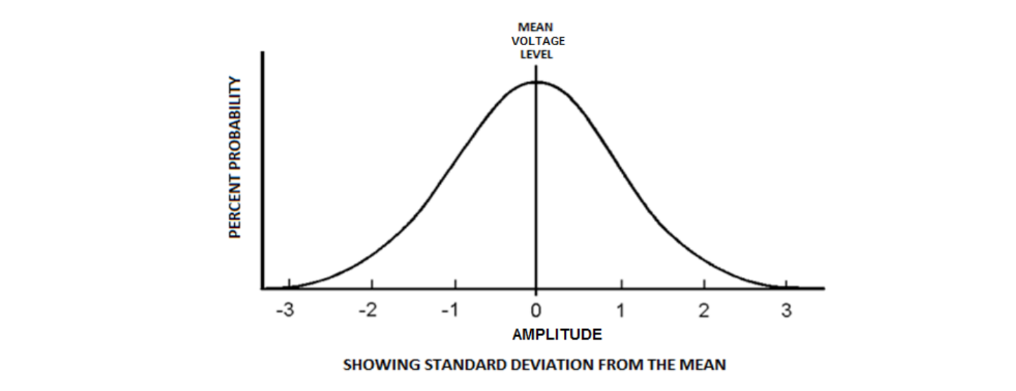
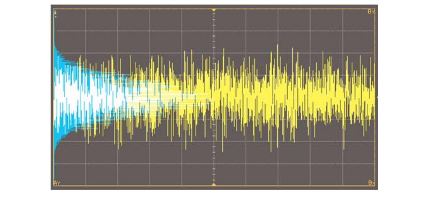
An AWGN signal has both positive and negative voltage values, with a mean value of zero. The following diagram shows how it would be displayed in the time domain on an oscilloscope, with its statistical analysis, the Gaussian curve, superimposed upon it in blue. The higher power positive and negative peaks are less likely to occur, so lie at the extreme ends of the probability curve, at high sigma values.
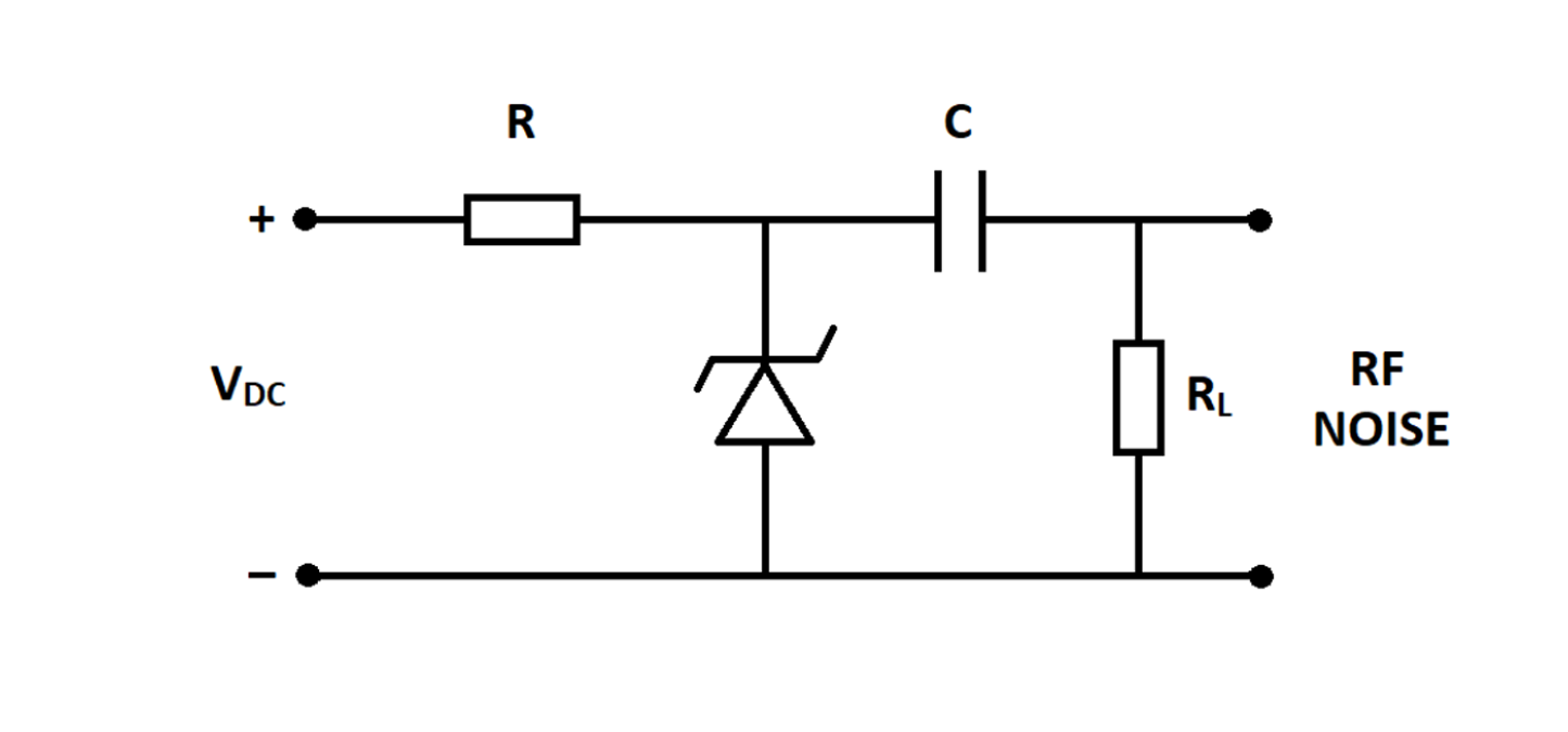
Practical AWGN can be generated using a reverse biased zener diode. When a high breakdown voltage is applied, the diode emits avalanche noise, which can be regarded as being a close approximation to AWGN. Doping, or the introduction of impurities in the semiconductor material, can be used to alter the breakdown voltage and to improve the frequency response of the output.
A resistor can also be used, which by its nature directly generates thermal noise. However, even though this is exactly the type of noise that RF engineers are trying to mitigate against, reverse biased zener diodes are more commonly used because they have a broader frequency spectrum and a Gaussian distribution. A typical bias circuit is shown below.
The resultant RF noise is then amplified in order to give a meaningful output which can then be packaged in either a module or an instrument. A simple instrument could contain an input port for the incoming signal, a combiner to add the noise, and individual attenuators for both the signal and the noise in order to set the required signal to noise ratio at the output port.
A digital signal processor (DSP) can also be used to create AWGN, whereby an algorithm which produces a stream of random numbers with a Gaussian distribution is added to the incoming signal. Although an expensive method, the advantage of using a DSP is that it provides speed and versatility, as they can be easily programmed to change the signal characteristics.
It is an unavoidable fact that all components within a system generate their own internal noise. Noise figure puts a value on this, and is essentially an indication of the degradation of signal to noise ratio at the output compared to the signal to noise ratio at the input, or the amount of noise added to the system by the device under test. In the following example the device under test is an amplifier with a gain of 20dB.
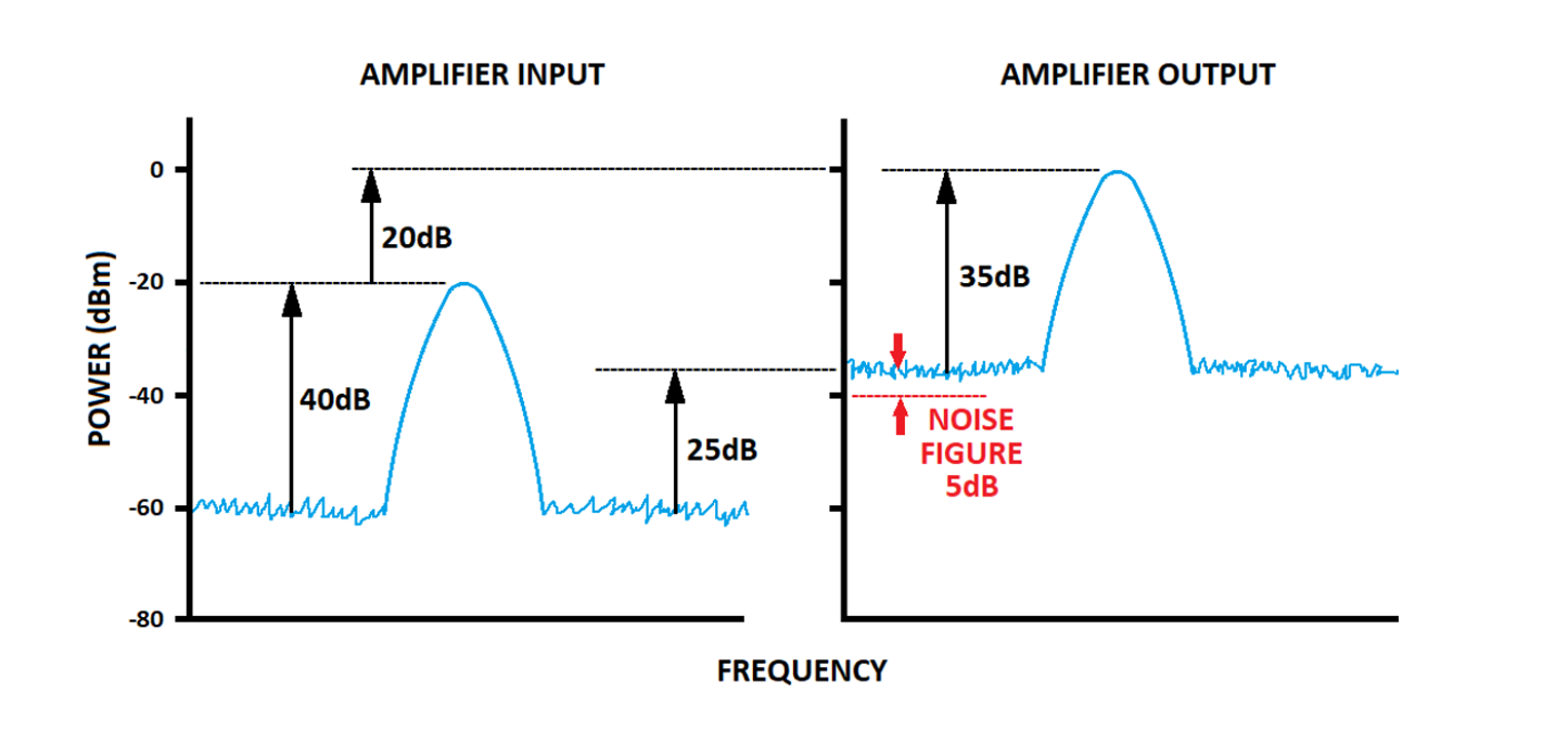
The output signal is 20dB greater than the input signal, as expected. But the output noise level would only be 20dB above the input noise level if this was a perfect amplifier, which can of course never be the case. In this example the noise floor has risen by 25dB, so the noise figure of the amplifier is 5dB.
It is of particular importance to engineers who design RF receivers and amplifiers, as the lower the noise figure the better the performance. Today’s highly sensitive receivers must be capable of amplifying very low strength signals. The low noise amplifiers (LNAs) used for these applications must also have very low noise figures, otherwise an excess amount of noise generated within the amplifier itself could swamp out the received signal.
Noise Figure, NF, is derived from Noise Factor, F, which is the signal to noise ratio at the input divided by the signal to noise ratio at the output of the device under test.
F = Si/Ni So/No
Due to the fact that noise will be added by the device under test, the value of F will always be greater than 1.
As gain (G) is
G = So/Si
the above equation can be re-written as:
F = No / (Ni · G)
NF is simply F expressed in terms of decibels.
NF = 10 log10(F)
Noise sources which produce accurately known levels of AWGN are required to find the noise figure of a DUT, and their outputs are expressed in terms of excess noise ratio, or ENR. When the source is switched off it will output the thermal noise floor of -174dBm/Hz, and when switched on the output will increase by the ENR, measured in dB.
The noise source manufacturer will provide calibrated ENR values across its frequency band. The following diagram shows how a noise figure meter is used.
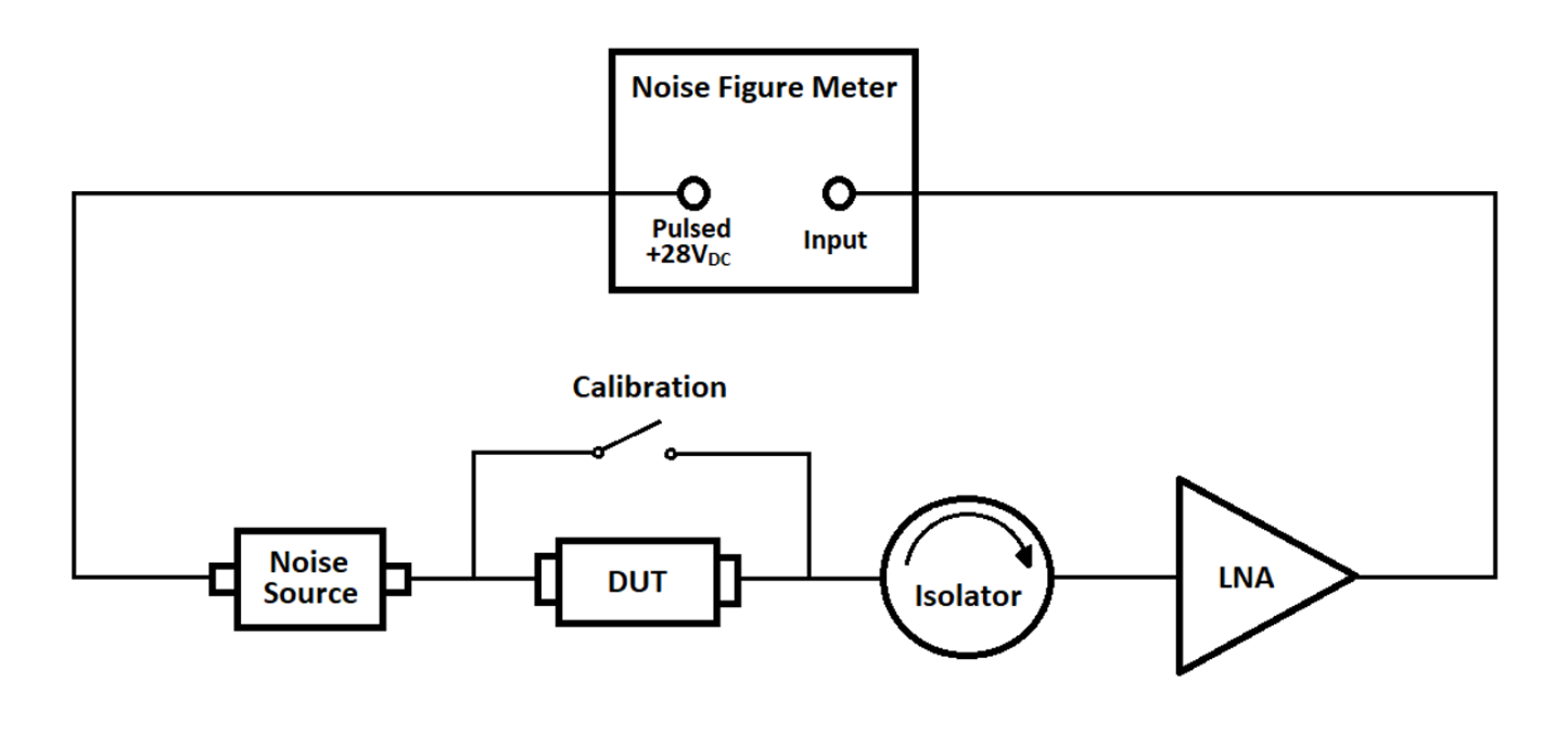
The isolator is used to reduce reflections and therefore improve VSWR, and the low noise amplifier, or LNA, is used to reduce the noise in the test setup.
First of all the noise source ENR values are input into the instrument across its frequency band. It provides a pulsed power supply to the noise source, and measures the ratio of the output noise power of a DUT when connected to a hot load (noise source switched on), and when connected to a cold load (noise source switched off). This ratio is called the Y-Factor,
Y = DUT output noise power with noise diode on DUT output noise power with noise diode off
The meter uses this value to calculate the noise figure,
NF = ENR − 10 log10(Y − 1)
The method has two steps. The first is calibration, where a reference level is established by finding the noise figure of the test setup without the DUT present, and the second step is a repeat of the first with the DUT inserted.
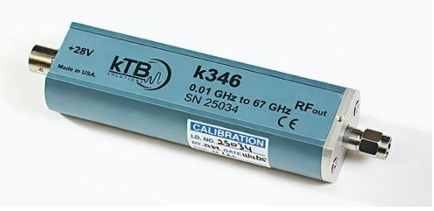
A typical calibrated noise source is shown below: